
QTQt displayer is a tool for displaying the results of data inversion using the QTQt software developed by K. Gallagher (Gallagher 2012).
Without strictly following it, it comes close to the recommendations made in the article (U-Th)/He chronology: Part 2. Considerations for evaluating, integrating, and interpreting conventional individual aliquot data (Flowers et al. 2023)
This tool is developed in python and is available as code (.py) or as a stand-alone application (.exe) running on Windows.
Citation: as this software is not published in the form of an academic article, you can refer to it in your articles in main text body (or in the acknowledgements following the publisher’s recommendations) as follows: “made with QTQt displayer (A. Derycke) available on https://deryckehub.ovh”.
Section:
Downloading :
Version :
- V0.4.4 (11/2024) : correction of bugs 1 to 3
- V0.4.3 (10/2024) : extension of the maximum number of samples (from 10 to 50) and improvement of the colour selection window
- V0.4.2 (10/2024) : display of resamples (if available) and addition of the legend for FTs
- V0.4 (09/2024) : corrected the bug displaying percents t(T) and added the display of He and FT data resampling
- V0.3.3.3 (07/2024) : file extensions managed for older versions of QTQt
- V0.3.3 : correction of various bugs
- V0.3 : added ‘right-click’ options on graphics and vertical profile management
- V0.2 : choice of sample colour management and multi-data files added
- V0.1 : serial file processing and graphical user interface added
Application :
Is the compiled application only available on Windows (compilation problems on MacOS)

QTQt displayer (.exe)
Helps folder :
Folder to place with the .exe or .py to be able to access certain Help for the graphics present on the interface. This Help can be accessed by right-clicking.
QTQt displayer Help
Python code :
The python source code is also available at GitHub official and as a Jupyter notebook:
QTQt displayer (.py)

QTQt displayer (Jupyter)
Tutorial and operation :
To work, QTQt displayer relies on the file generated by QTQt at the end of an inversion, which contains the main results. The file is called “runname.txt” (or “QTQt.txt” if you have not named the run) and if you leave the default settings, it is located in the same folder as your sample files.
Interface :
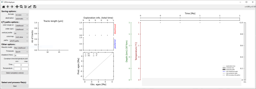
Once the application or code has been launched (which takes several seconds for optimisation reasons) you are presented with an interface with :
- options on the left which can be preset before processing a file, or modified after displaying the figure to update it
- figure on the right which you can interact with using the tools at the top (change scales, move around the chart, change colours, etc.) or by right-clicking on the charts (contextual help, data export).
How to use :
- start/end a data inversion with QTQt
- start QTQt displayer
- select the formatting options on the left (optional)
- click on “Start” at the bottom to select the file(s) to be processed. Note: figure creation is slower than with QTQt and depends on the number of iterations:
- > 100 000′ iterations can take several seconds
- > 1,000,000′ iterations can take several minutes
Backup and export :
There are two ways of recording the figure(s):
- after the creation of the figure by clicking on the “save” logo at the top, but this only saves one figure.
- before the creation of the figure by switching the “formats” option to the one you want. In this case, if you select several results from different QTQt runs, this will generate one figure per run (processing in series following runs).
Furthermore, if you want to retrieve the “predicted ages vs observed ages” data in a table, you can extract it to a .csv table by right-clicking on the graph.
How to read the figure :
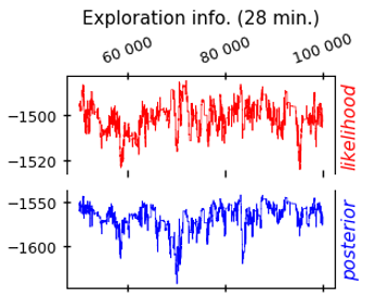
Exploration info. (temps) : total duration of reversal (burn-in + post-burn-in).
Likelihood et posterior : evolution of the two parameters calculated by QTQt during the inversion (post-burn-in iteration), their trend making it possible to assess the reliability of the inversion.
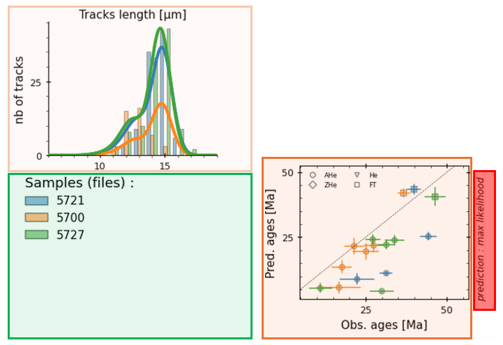
Samples et data: in green on the image, the list of samples and their corresponding colours (one file = one sample). In red, the QTQt model used for predictions (opt. results model). In orange, the observed vs predicted He and FT data. For the lengths (top left), the bars are the observed data and the solid lines are the predicted data.
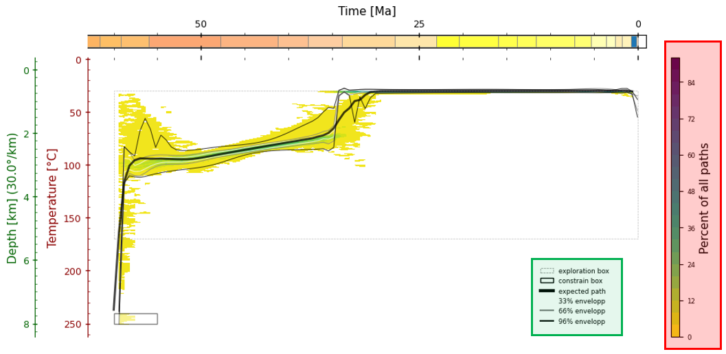
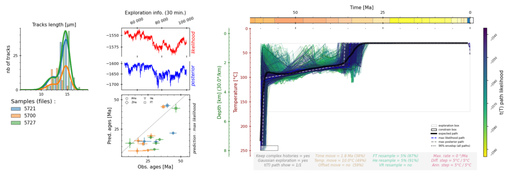
Graph time — temperature : on the right (in red) legend of the colourimetry of the paths. At the bottom (green insert) is a legend of the paths shown in the figure and on the left (green axis) the temperature-depth equivalence for a given temperature gradient.
Inversion parameters : summary of data inversion parameters

Options available:
Saving options :
- formats : automatic export format for the figure after it has been created (“no save” = no automatic saving)
- destination : export destination folder saved automatically (“automatic” = same folder and name as the input run file)
t(T) paths options :
- ranking parameter : according to which the colouring of t(T) paths is applied
- likelihood : data reproducibility index
- posterieur : likelihood weighted by path complexity
- iteration : position of appearance during inversion
- order (opt.) :z” order of path representation. The same value as the “ranking parameter” is automatically selected to rank the paths with the highest value above (the most visible).
- vertical profile : is used to define the type of path displayed in the case of a vertical profile (different path t(T))
- colormap : range of colours to represent the ranking parameter. Note that the “mid values” and “extrem values” colours are based on the recommendations of Scientific Color Map (published in Crameri et al., 2020).
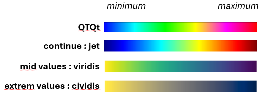
- paths : choice of path representations
- all path : representation of the set of paths t(T)
- percentage : heat map of the percentage of paths passing through a temperature range (1°C) for a given time, as well as the 33, 66 and 99% envelope of the paths
- envelop : covering 96% of the roads
Other options :
- resutls model : model of predicted data chosen to be represented in the accompanying graphs
- maximum likelihood : best “observed vs. predicted” match
- maximum posterior : best “observed vs predicted” match for a simple path
- expected : prediction of the estimated mean path deduced from data inversion
- timescale : choice of resolution of the geological time scale represented(International Chronostratigraphic Chart) accessible through pyrolite
- gradient : input of the thermal gradient in °/km to represent the temperature-depth relationship
- constrain t(T) plot : manual entry of the limits of the t(T) graph (useful in the case of serial export of several inversions)
- select sample(s) color(s) : selection of the colours used to represent the ages and lengths of fission tracks, it is possible to define them before processing a file. Note: in the case of serial processing of several inversions, a memory system allows the colour of the samples from one inversion to be transmitted at the same time as the name.
Comments and bug reports :
V0.4.3 :
- bug 1 : on envelope creation case init = 0
- bug 2 : on the case eU resample but not all samples have He
- bug 3 : save as pdf after compilation – missing librairy matplotlib backends